Kolmogorov–Arnold and Kolmogorov–Gabor Models Their Relationship and Influence on Modern Neural Networks Introduction Ko...
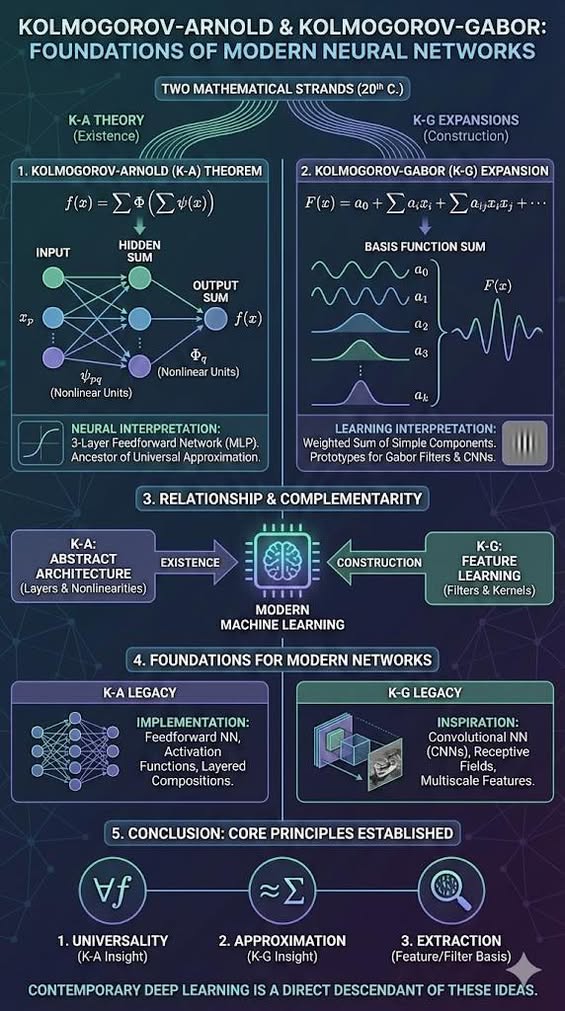
Kolmogorov–Arnold and Kolmogorov–Gabor Models Their Relationship and Influence on Modern Neural Networks Introduction Kolmogorov–Arnold superposition theory and Kolmogorov–Gabor functional expansions provided the conceptual bedrock for modern neural networks. While their adoption was separated by the 1987–1993 “AI Winter”—triggered by the crash of the expert-systems market and symbolic AI disillusionment—they ultimately converge on one central idea: complex multivariate functions can be constructed from combinations of simple functional units. This article explains the relationship between these two frameworks and how they informed the structure and capability of today’s neural-network architectures. ⸻ Personal Note: I myself applied the Kolmogorov Gabor model in a Socio-Economic planning application for Strategic Planning of Telecommunications Networks and Applications in the late 1980’s as part of my Doctoral Studies. Related… https://www.facebook.com/share/p/1DM8MRYf9g/?mibextid=wwXIfr ⸻ 1. The Kolmogorov–Arnold Superposition Theorem In 1957, Andrey Kolmogorov proved a now-famous result (refined shortly after by Vladimir Arnold) stating that every multivariate continuous function can be expressed as a finite composition of continuous univariate functions and addition. The Mathematical Formulation For any continuous function f : [0,1]^n -> R there exist continuous functions Φ_q and ψ_pq such that: f(x_1, ..., x_n) = sum_{q=1}^{2n+1} Φ_q( sum_{p=1}^n ψ_{pq}(x_p) ) Neural-Network Interpretation The structure of this expression corresponds to a three-layer feedforward neural network: 1. Input variables x_p pass through univariate nonlinear transformations ψ_pq. 2. These transformed values are summed. 3. A second nonlinear function Φ_q is applied to each sum, and then all outputs are summed to produce f(x). This representation contains exactly the elements of modern multilayer perceptrons: nonlinear activation functions and weighted summation units arranged in layers. Kolmogorov’s result is widely regarded as the conceptual ancestor of the Universal Approximation Theorem. Later researchers—including Hecht-Nielsen (1987), Cybenko (1989), and Hornik (1991)—explicitly cited the Kolmogorov–Arnold theorem as the mathematical basis showing that neural networks with standard activation functions can approximate any continuous function on compact sets. ⸻ 2. The Kolmogorov–Gabor Functional Expansion Decades before the modern neural-network era, both Kolmogorov (in the 1930s) and Dennis Gabor (in 1946) developed approaches for representing arbitrary functional relationships as series expansions. The Mathematical Formulation A generic Kolmogorov–Gabor expansion expresses a multivariate function as: F(x_1, ..., x_n) = a_0 + sum_i a_i x_i + sum_{i,j} a_{ij} x_i x_j + sum_{i,j,k} a_{ijk} x_i x_j x_k + ... Kolmogorov used these polynomial-like expansions in modeling complex physical and biological systems. Gabor, however, introduced a different kind of basis, using sinusoidal or Gaussian-modulated functions. These “Gabor functions” later became: • Early models of receptive fields in the mammalian visual cortex • Foundations of time-frequency analysis • Prototypes of convolutional filters used in early image-processing systems Learning Interpretation The expansion represents a function as a weighted sum of simple components. Learning consists of estimating weights such as a_i or a_ij. This is structurally identical to how linear models, kernel machines, and neural networks assign trained weights to basis functions or learned feature detectors. Thus the Kolmogorov–Gabor programme introduced the idea that: • A function can be represented by combining simple basis functions. • Feature extraction is equivalent to defining or learning these basis functions. • Learning algorithms adjust the coefficients of these components. These principles prefigure many aspects of convolutional networks, kernel methods, and dictionary learning. ⸻ 3. Relationship Between the Two Approaches Both Kolmogorov–Arnold and Kolmogorov–Gabor models address the same conceptual challenge: How can high-dimensional functions be decomposed into simpler parts? But they approach the question from different perspectives. Kolmogorov–Arnold provided a theorem of existence: any continuous function can be represented by layered univariate nonlinear functions and addition. Kolmogorov–Gabor provided a method of construction: explicit basis functions (polynomials, sinusoids, Gaussians) that can approximate real-world functions in practice. Complementarity: • Kolmogorov–Arnold shows that a network of simple nonlinear units is sufficient to represent any continuous function. • Kolmogorov–Gabor shows how real-world functions can be approximated using explicit, structured basis sets. Together they foreshadow the two halves of modern machine learning: 1. Architecture — the existence of layered nonlinear models 2. Feature learning — expansions, basis functions, filters, kernels ⸻ 4. Foundations for Modern Neural Networks 4.1 Neural Networks as Implementations of Kolmogorov–Arnold The modern feedforward neural network uses exactly the components found in the Kolmogorov–Arnold decomposition: • Scalar nonlinear activation functions • Weighted sums • Layered compositions This is why Kolmogorov’s theorem is recognized as the first universal approximation result—decades before the neural-network field formally defined the concept. The universal approximation theorems of the late 1980s and early 1990s generalized and operationalized Kolmogorov’s insight, proving that networks with sigmoidal or ReLU-type activations can approximate any continuous function under broad conditions. 4.2 Convolutional Neural Networks and the Gabor Legacy Gabor’s work introduced localized sinusoidal and Gaussian-modulated basis functions, which later became known as Gabor filters. These filters resemble the receptive fields discovered by Hubel and Wiesel in the visual cortex and closely match the filters learned automatically in the early layers of modern convolutional neural networks. Thus: • Kolmogorov–Gabor expansions inspired the structure of convolutional filters. • Gabor bases are still used to analyze and visualize learned CNN features. • Gabor’s time-frequency approach underlies the idea of localized, multiscale feature extraction. Gabor’s contribution is therefore foundational to representation learning, especially in vision and signal processing. 4.3 The “Lost” Implementation: Ivakhnenko and the Group Method As documented in the historical survey by Schmidhuber (2015), the history of deep learning often suffers from a form of amnesia, frequently attributing the invention of deep networks solely to later breakthroughs of the 1980s and 2000s. In reality, the first deep-learning networks—developed by Alexey Ivakhnenko in 1965 using the Group Method of Data Handling (GMDH)—were direct engineering implementations of Kolmogorov–Gabor polynomial expansions. These mathematical frameworks were not merely abstract inspirations; they served as the literal blueprints for the first working deep-learning algorithms, a legacy often overshadowed by the AI Winter of 1987–1993 that followed. ⸻ 5. Conclusion Kolmogorov’s decomposition demonstrated that any continuous multivariate function can be built from layered combinations of simple univariate nonlinearities—anticipating the architecture and expressive power of modern neural networks. Gabor’s functional expansions, along with Kolmogorov’s earlier polynomial expansions, illustrated how real-world functions can be approximated by sums of basis functions—anticipating learned filters, convolutional architectures, and kernel methods. Together, these two bodies of work established core principles of modern deep learning: 1. Universality — neural networks can represent any continuous function. 2. Approximation — functions can be approximated by weighted sums of simple basis elements. 3. Extraction — feature extraction and filter decomposition are fundamental to perception and learning. Modern neural networks, from multilayer perceptrons to convolutional architectures, descend directly from these ideas. ⸻ References Kolmogorov–Arnold Theory 1. A. N. Kolmogorov (1957). “On the Representation of Continuous Functions of Several Variables by Superposition of Continuous Functions of One Variable and Addition.” Doklady Akademii Nauk SSSR. 2. V. I. Arnold (1957–1958). “On Functions of Three Variables.” Doklady Akademii Nauk SSSR. 3. R. Hecht-Nielsen (1987). “Kolmogorov’s Mapping Neural Network Existence Theorem.” Proc. IEEE Int. Conf. Neural Networks. 4. G. Cybenko (1989). “Approximation by Superpositions of a Sigmoidal Function.” Mathematics of Control, Signals and Systems. 5. K. Hornik (1991). “Approximation Capabilities of Multilayer Feedforward Networks.” Neural Networks. Kolmogorov–Gabor Expansions and Gabor Functions 6. D. Gabor (1946). “Theory of Communication.” Journal of the IEE. 7. A. N. Kolmogorov (1930s–1950s). Papers on polynomial and functional expansions. 8. J. Daugman (1985). “Uncertainty Relation for Resolution in Space, Spatial Frequency, and Orientation.” J. Optical Society of America. 9. J. Daugman (1988). “Complete Discrete 2D Gabor Transform by Neural Networks.” Int. Journal of Neural Systems. Neural Network Development 10. Y. LeCun et al. (1998). “Gradient-Based Learning Applied to Document Recognition.” Proc. IEEE. 11. I. Goodfellow, Y. Bengio, A. Courville (2016). “Deep Learning.” MIT Press. 12. U. Montufar et al. (2014). “On the Number of Linear Regions of Deep Neural Networks.” NeurIPS. 13. J. Schmidhuber (2015). “Deep Learning in Neural Networks: An Overview.” Neural Networks 61: 85–117.